Sigmoid neurons

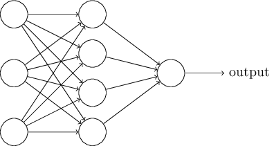
Learning algorithms sound terrific. But how can we devise such algorithms for a neural network? Suppose we have a network of perceptrons that we’d like to use to learn to solve some problem. For example, the inputs to the network might be the raw pixel data from a scanned, handwritten image of a digit. And we’d like the network to learn weights and biases so that the output from the network correctly classifies the digit. To see how learning might work, suppose we make a small change in some weight (or bias) in the network. What we’d like is for this small change in weight to cause only a small corresponding change in the output from the network. As we’ll see in a moment, this property will make learning possible. Schematically, here’s what we want (obviously this network is too simple to do handwriting recognition!):

If it were true that a small change in a weight (or bias) causes only a small change in output, then we could use this fact to modify the weights and biases to get our network to behave more in the manner we want. For example, suppose the network was mistakenly classifying an image as an “8” when it should be a “9”. We could figure out how to make a small change in the weights and biases so the network gets a little closer to classifying the image as a “9”. And then we’d repeat this, changing the weights and biases over and over to produce better and better output. The network would be learning.

The problem is that this isn’t what happens when our network contains perceptrons. In fact, a small change in the weights or bias of any single perceptron in the network can sometimes cause the output of that perceptron to completely flip, say from 0 to 1. That flip may then cause the behaviour of the rest of the network to completely change in some very complicated way. So while your “9” might now be classified correctly, the behaviour of the network on all the other images is likely to have completely changed in some hard-to-control way. That makes it difficult to see how to gradually modify the weights and biases so that the network gets closer to the desired behaviour. Perhaps there’s some clever way of getting around this problem. But it’s not immediately obvious how we can get a network of perceptrons to learn.

We can overcome this problem by introducing a new type of artificial neuron called a sigmoid neuron. Sigmoid neurons are similar to perceptrons, but modified so that small changes in their weights and bias cause only a small change in their output. That’s the crucial fact which will allow a network of sigmoid neurons to learn.

Okay, let me describe the sigmoid neuron. We’ll depict sigmoid neurons in the same way we depicted perceptrons:

Just like a perceptron, the sigmoid neuron has inputs, x1,x2,…. But instead of being just 0 or 1, these inputs can also take on any values between 0 and 1. So, for instance, 0.638… is a valid input for a sigmoid neuron. Also just like a perceptron, the sigmoid neuron has weights for each input, w1,w2,…, and an overall bias, b. But the output is not 0 or 1. Instead, it’s σ(w⋅x+b), where σ is called the sigmoid function*, and is defined by:

σ(z)≡1/(1+e−z次方).         (3)

To put it all a little more explicitly, the output of a sigmoid neuron with inputs x1,x2,…, weights w1,w2,…, and bias b is

1/[1+exp(−∑jwjxj−b)].            (4).

At first sight, sigmoid neurons appear very different to perceptrons. The algebraic form of the sigmoid function may seem opaque and forbidding if you’re not already familiar with it. In fact, there are many similarities between perceptrons and sigmoid neurons, and the algebraic form of the sigmoid function turns out to be more of a technical detail than a true barrier to understanding.

To understand the similarity to the perceptron model, suppose z≡w⋅x+b is a large positive number. Then e−z≈0 and so σ(z)≈1. In other words, when z=w⋅x+b is large and positive, the output from the sigmoid neuron is approximately 1, just as it would have been for a perceptron. Suppose on the other hand that z=w⋅x+b is very negative. Then e−z→∞, and σ(z)≈0. So when z=w⋅x+b is very negative, the behaviour of a sigmoid neuron also closely approximates a perceptron. It’s only when w⋅x+b is of modest size that there’s much deviation from the perceptron model. sigmoid函数的作用，将w.x+b的巨大变化[-∞,+∞]映射到了很小的变化上[0,1]。

What about the algebraic form of σ? How can we understand that? In fact, the exact form of σ isn’t so important – what really matters is the shape of the function when plotted. Here’s the shape:

This shape is a smoothed out version of a step function:

If σ had in fact been a step function, then the sigmoid neuron would be a perceptron, since the output would be 1 or 0 depending on whether w⋅x+b was positive or negative. By using the actual σ function we get, as already implied above, a smoothed out perceptron. Indeed, it’s the smoothness of the σ function that is the crucial fact, not its detailed form. The smoothness of σ means that small changes Δwj in the weights and Δb in the bias will produce a small change Δoutput in the output from the neuron. In fact, calculus tells us that Δoutput is well approximated by

where the sum is over all the weights, wj, and ∂output/∂wj and ∂output/∂b denote partial derivatives偏导数 of the output with respect to wj and b, respectively. Don’t panic if you’re not comfortable with partial derivatives! While the expression above looks complicated, with all the partial derivatives, it’s actually saying something very simple (and which is very good news): Δoutput is a linear function of the changes Δwjand Δb in the weights and bias. This linearity makes it easy to choose small changes in the weights and biases to achieve any desired small change in the output. So while sigmoid neurons have much of the same qualitative behaviour as perceptrons, they make it much easier to figure out how changing the weights and biases will change the output.

If it’s the shape of σ which really matters, and not its exact form, then why use the particular form used for σ in Equation (3)? In fact, later in the book we will occasionally consider neurons where the output is f(w⋅x+b) for some other activation function激励函数 f(⋅). The main thing that changes when we use a different activation function is that the particular values for the partial derivatives偏导数 in Equation (5) change. It turns out that when we compute those partial derivatives later, using σ will simplify the algebra, simply because exponentials have lovely properties when differentiated. In any case, σ is commonly-used in work on neural nets, and is the activation function we’ll use most often in this book.

How should we interpret the output from a sigmoid neuron? Obviously, one big difference between perceptrons and sigmoid neurons is that sigmoid neurons don’t just output 0 or 1. They can have as output any real number between 0 and 1, so values such as 0.173… and 0.689… are legitimate outputs. This can be useful, for example, if we want to use the output value to represent the average intensity of the pixels in an image input to a neural network. But sometimes it can be a nuisance. Suppose we want the output from the network to indicate either “the input image is a 9” or “the input image is not a 9”. Obviously, it’d be easiest to do this if the output was a 0 or a 1, as in a perceptron. But in practice we can set up a convention to deal with this, for example, by deciding to interpret any output of at least 0.5 as indicating a “9”, and any output less than 0.5 as indicating “not a 9”. I’ll always explicitly state when we’re using such a convention, so it shouldn’t cause any confusion.  stimulate VS simulate

Exercises

• Sigmoid neurons simulating perceptrons, part I 
  Suppose we take all the weights and biases in a network of perceptrons, and multiply them by a positive constant, c>0. Show that the behaviour of the network doesn’t change.       c(w*x+b) >0  ==  w*x+b>0
• Sigmoid neurons simulating perceptrons, part II 
  Suppose we have the same setup as the last problem – a network of perceptrons. Suppose also that the overall input to the network of perceptrons has been chosen. We won’t need the actual input value, we just need the input to have been fixed. Suppose the weights and biases are such that w⋅x+b≠0 for the input x to any particular perceptron in the network. Now replace all the perceptrons in the network by sigmoid neurons, and multiply the weights and biases by a positive constant c>0. Show that in the limit as c→∞ the behaviour of this network of sigmoid neurons is exactly the same as the network of perceptrons. How can this fail when w⋅x+b=0 for one of the perceptrons?

The architecture of neural networks

In the next section I’ll introduce a neural network that can do a pretty good job classifying handwritten digits. In preparation for that, it helps to explain some terminology that lets us name different parts of a network. Suppose we have the network:

As mentioned earlier, the leftmost layer in this network is called the input layer, and the neurons within the layer are called input neurons. The rightmost or output layer contains the output neurons, or, as in this case, a single output neuron. The middle layer is called a hidden layer, since the neurons in this layer are neither inputs nor outputs. The term “hidden” perhaps sounds a little mysterious – the first time I heard the term I thought it must have some deep philosophical or mathematical significance – but it really means nothing more than “not an input or an output”. The network above has just a single hidden layer, but some networks have multiple hidden layers. For example, the following four-layer network has two hidden layers:

Somewhat confusingly, and for historical reasons, such multiple layer networks are sometimes called multilayer perceptrons orMLPs, despite being made up of sigmoid neurons, not perceptrons. I’m not going to use the MLP terminology in this book, since I think it’s confusing, but wanted to warn you of its existence.

The design of the input and output layers in a network is often straightforward. For example, suppose we’re trying to determine whether a handwritten image depicts a “9” or not. A natural way to design the network is to encode the intensities强度 of the image pixels into the input neurons. If the image is a 64 by 64 greyscale灰度的 image, then we’d have 4,096=64×64 input neurons, with the intensities scaled appropriately between 0 and 1. The output layer will contain just a single neuron, with output values of less than 0.5 indicating “input image is not a 9”, and values greater than 0.5 indicating “input image is a 9 “.

While the design of the input and output layers of a neural network is often straightforward, there can be quite an art to the design of the hidden layers. In particular, it’s not possible to sum up the design process for the hidden layers with a few simple rules of thumb特别是用几个简单的经验法则来总结隐藏层的设计过程是不可能的. Instead, neural networks researchers have developed many design heuristics for the hidden layers, which help people get the behaviour they want out of their nets. For example, such heuristics can be used to help determine how to trade off the number of hidden layers against the time required to train the network. We’ll meet several such design heuristics later in this book.

Up to now, we’ve been discussing neural networks where the output from one layer is used as input to the next layer. Such networks are called feedforward neural networks. This means there are no loops in the network – information is always fed forward, never fed back. If we did have loops, we’d end up with situations where the input to the σ function depended on the output. That’d be hard to make sense of, and so we don’t allow such loops.

However, there are other models of artificial neural networks in which feedback loops are possible. These models are called recurrent neural networks. The idea in these models is to have neurons which fire for some limited duration of time, before becoming quiescent. That firing can stimulate other neurons, which may fire a little while later, also for a limited duration. That causes still more neurons to fire, and so over time we get a cascade of neurons firing. Loops don’t cause problems in such a model, since a neuron’s output only affects its input at some later time, not instantaneously.

Recurrent neural nets have been less influential than feedforward networks, in part because the learning algorithms for recurrent nets are (at least to date) less powerful. But recurrent networks are still extremely interesting. They’re much closer in spirit to how our brains work than feedforward networks. And it’s possible that recurrent networks can solve important problems which can only be solved with great difficulty by feedforward networks. However, to limit our scope, in this book we’re going to concentrate on the more widely-used feedforward networks.

A simple network to classify handwritten digits

Having defined neural networks, let’s return to handwriting recognition. We can split the problem of recognizing handwritten digits into two sub-problems. First, we’d like a way of breaking an image containing many digits into a sequence of separate images, each containing a single digit. For example, we’d like to break the image

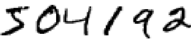into six separate images,

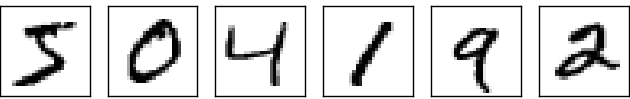We humans solve this segmentation problem with ease, but it’s challenging for a computer program to correctly break up the image. Once the image has been segmented, the program then needs to classify each individual digit. So, for instance, we’d like our program to recognize that the first digit above,

is a 5.

We’ll focus on writing a program to solve the second problem, that is, classifying individual digits. We do this because it turns out that the segmentation problem is not so difficult to solve, once you have a good way of classifying individual digits. There are many approaches to solving the segmentation problem. One approach is to trial many different ways of segmenting the image, using the individual digit classifier to score each trial segmentation. A trial segmentation gets a high score if the individual digit classifier is confident of its classification in all segments, and a low score if the classifier is having a lot of trouble in one or more segments. The idea is that if the classifier is having trouble somewhere, then it’s probably having trouble because the segmentation has been chosen incorrectly. This idea and other variations can be used to solve the segmentation problem quite well. So instead of worrying about segmentation we’ll concentrate on developing a neural network which can solve the more interesting and difficult problem, namely, recognizing individual handwritten digits.

To recognize individual digits we will use a three-layer neural network:

The input layer of the network contains neurons encoding the values of the input pixels. As discussed in the next section, our training data for the network will consist of many 28 by 28 pixel images of scanned handwritten digits, and so the input layer contains 784=28×28 neurons. For simplicity I’ve omitted most of the 784 input neurons in the diagram above. The input pixels are greyscale, with a value of 0.0 representing white, a value of 1.0 representing black, and in between values representing gradually darkening shades of grey.

The second layer of the network is a hidden layer. We denote the number of neurons in this hidden layer by n, and we’ll experiment with different values for n. The example shown illustrates a small hidden layer, containing just n=15 neurons.

The output layer of the network contains 10 neurons. If the first neuron fires, i.e., has an output ≈1, then that will indicate that the network thinks the digit is a 0. If the second neuron fires then that will indicate that the network thinks the digit is a 1. And so on. A little more precisely, we number the output neurons from 0 through 9, and figure out which neuron has the highest activation value( what does this mean? what is activation value). If that neuron is, say, neuron number 6, then our network will guess that the input digit was a 6. And so on for the other output neurons.

You might wonder why we use 10 output neurons. After all, the goal of the network is to tell us which digit (0,1,2,…,9) corresponds to the input image. A seemingly natural way of doing that is to use just 4 output neurons, treating each neuron as taking on a binary value, depending on whether the neuron’s output is closer to 0 or to 1. Four neurons are enough to encode the answer, since 2⁴=16 is more than the 10 possible values for the input digit. Why should our network use 10 neurons instead? Isn’t that inefficient? The ultimate justification is empirical: we can try out both network designs, and it turns out that, for this particular problem, the network with 10 output neurons learns to recognize digits better than the network with 4 output neurons. But that leaves us wondering why using 10 output neurons works better. Is there some heuristic启发性 that would tell us in advance that we should use the 10-output encoding instead of the 4-output encoding?

To understand why we do this, it helps to think about what the neural network is doing from first principles. Consider first the case where we use 10 output neurons. Let’s concentrate on the first output neuron, the one that’s trying to decide whether or not the digit is a 0. It does this by weighing up权衡 evidence from the hidden layer of neurons. What are those hidden neurons doing? Well, just suppose for the sake of argument论据 that the first neuron in the hidden layer detects whether or not an image like the following is present:       sake 日本清酒 VS sane adj.明智的; for the sake of 为了。。

It can do this by heavily weighting input pixels which overlap with the image, and only lightly weighting the other inputs. In a similar way, let’s suppose for the sake of argument that the second, third, and fourth neurons in the hidden layer detect whether or not the following images are present:

As you may have guessed, these four images together make up the 0 image that we saw in the line of digits shown earlier:

So if all four of these hidden neurons are firing then we can conclude that the digit is a 0. Of course, that’s not the only sort of evidence we can use to conclude that the image was a 0 – we could legitimately get a 0 in many other ways (say, through translations of the above images, or slight distortions). But it seems safe to say that at least in this case we’d conclude that the input was a 0.

Supposing the neural network functions in this way, we can give a plausible似乎合理的 explanation for why it’s better to have 10 outputs from the network, rather than 4. If we had 4 outputs, then the first output neuron would be trying to decide what the most significant bit of the digit was. And there’s no easy way to relate that most significant bit to simple shapes like those shown above. It’s hard to imagine that there’s any good historical reason the component shapes of the digit will be closely related to (say) the most significant bit in the output.

Now, with all that said, this is all just a heuristic启发式的. Nothing says that the three-layer neural network has to operate in the way I described, with the hidden neurons detecting simple component shapes. Maybe a clever learning algorithm will find some assignment of weights that lets us use only 4 output neurons. But as a heuristic the way of thinking I’ve described works pretty well, and can save you a lot of time in designing good neural network architectures.

Exercise

• There is a way of determining the bitwise representation of a digit 确定数字的按位表示 通过by adding an extra layer to the three-layer network above. The extra layer converts the output from the previous layer into a binary representation, as illustrated in the figure below. Find a set of weights and biases for the new output layer. Assume that the first 3 layers of neurons are such that the correct output in the third layer (i.e., the old output layer) has activation at least 0.99, and incorrect outputs have activation less than 0.01.